Imagine you have data that shows how the price of a house depends on factors like its size, number of rooms, and location. Linear regression is like your magical tool to understand and predict this relationship. Here's the easy breakdown:

1. What is Linear Regression?
   Linear regression is a way to find a straight line that best shows how one thing (like house price) is affected by another thing (like house size). At its core, linear regression is a technique to understand and predict how one thing (let's call it "Y") is related to one or more other things (let's call them "Xs"). You can think of Y as the result of some process, and Xs as the factors that influence that result.

2. The Players
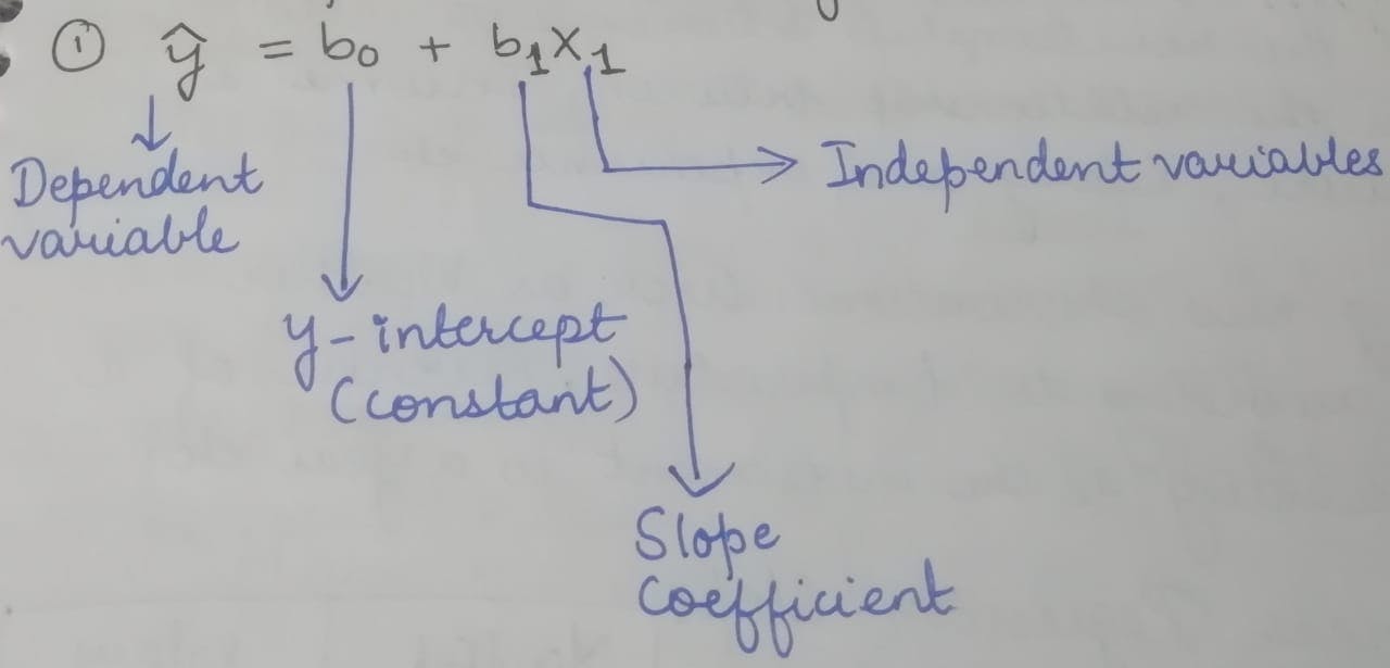
   In this game, you have 2 types of variables:

   Dependent Variable (Y): This is the thing you're trying to predict. It's the outcome or result you're interested in. For example, in real estate, this could be the house price.

   Independent Variables (Xs): These are the factors you believe influence the dependent variable. For house prices, it could be the number of rooms, square footage, or location.

3. The Straight Line or Regression Line
   Imagine you want to draw a line on a graph that predicts house prices. Linear regression helps you find the best-fitting line.
   In simple linear regression, this is a straight line that represents the relationship between the independent variable (X) and the dependent variable (Y). In multiple linear regression, it's a hyperplane.

4. Slope and Intercept
   The line has a slope and an intercept. The slope tells you how much the house price changes for every extra unit of house size. The intercept is the house price when the house size is zero (which doesn't make much sense in the real world).
   The slope (b₁) represents how much Y changes for a one-unit change in X, and the intercept (b₀) is the value of Y when X is zero.

   Slope (b₁): This tells you how much Y changes when one of your Xs changes. For example, if you're predicting house prices, it might tell you that for every extra square foot, the price goes up by a certain amount.

   Intercept (b₀): This is where your line crosses the Y-axis. It represents the value of Y when all your Xs are zero. In our house price example, it might be the price of a house with zero square footage (which doesn't exist in reality).

5. Residuals(Errors)
   Predictions are rarely perfect. Errors happen. Linear regression helps you find the line that minimizes the difference between your predictions and the actual values. It's all about getting as close as possible.

   These are the differences between the actual Y values and the predicted Y values. The goal is to minimize these residuals, which indicate the model's accuracy.

6. Ordinary Least Squares(OLS)
   Linear regression typically uses the OLS method to find the best-fitting line. It minimizes the sum of squared residuals, finding the line that minimizes the overall error.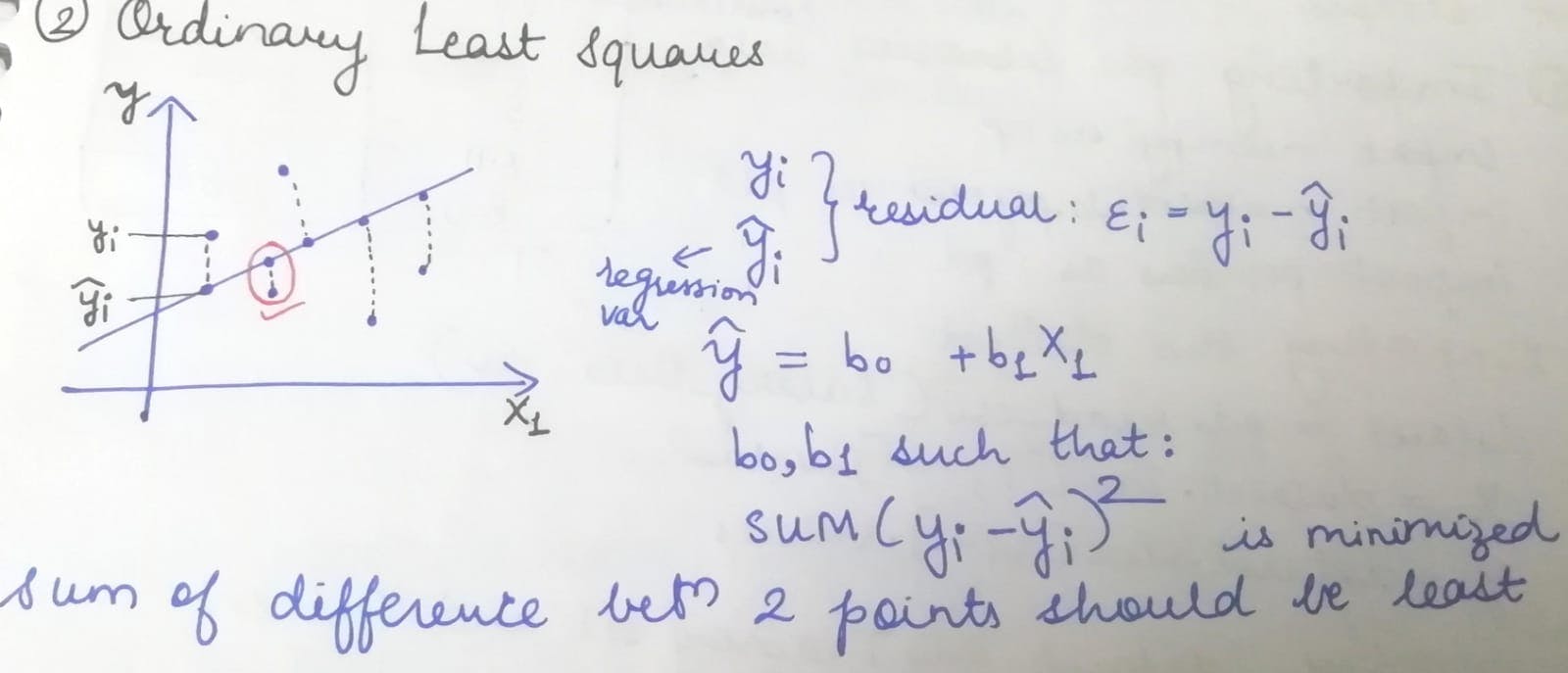

   

7. Assumptions of Linear Regression

Linearity:
Assumption:
This assumption means that the relationship between your independent variables (the Xs) and the dependent variable (Y) is a straight line. In other words, a change in X results in a consistent change in Y.

Example:
If you're predicting house prices, the linearity assumption suggests that adding one more bedroom should always result in a similar increase in the price, regardless of the house's size.

Independence of Errors:
Assumption:
This means that the errors (the differences between your predictions and the actual values) should not be connected. Each prediction's error should be unique and not influenced by the errors of other predictions.

Example:
Let's say you're forecasting stock prices. If one prediction's error is due to a sudden market event, it shouldn't affect the errors of other predictions for unrelated stocks.

Homoscedasticity (Constant Variance):
Assumption:
This assumption implies that the spread of errors should be roughly the same across all values of your independent variables (Xs). In simple terms, the variability of errors should be consistent.
*
Example:*
If you're studying the relationship between rainfall (X) and crop yield (Y), homoscedasticity means that the variation in crop yield should be similar whether you're in a region with high or low rainfall.

Multivariate Normality:
Assumption:
This assumption requires that the errors (the differences between predictions and actual values) follow a bell-shaped curve, similar to a normal distribution. It suggests that most errors are small and extreme errors are rare.

Example:
If you're examining test scores (Y) based on study time (X), the normal distribution assumption means that most students' test score errors will be small, with only a few students experiencing very high or very low errors.

No or Little Multicollinearity:
Assumption:
This assumption requires that the independent variables (Xs) should not be highly correlated or related to each other. In other words, they should bring unique and distinct information to the model.

Example:
Suppose you're predicting a car's fuel efficiency (miles per gallon, or mpg). If you include both engine size (measured in litres) and number of cylinders as independent variables, and they are highly correlated (as a larger engine often means more cylinders), it can cause multicollinearity issues. It becomes challenging for the model to distinguish their individual effects on fuel efficiency.

No Endogeneity
Assumption:
Endogeneity means that there should be no causal relationship between the independent variables (Xs) and the dependent variable (Y) that goes in the direction from Y to Xs. In simpler terms, your Xs should not be influenced by the thing you're trying to predict.

Example:
Let's say you're studying the impact of education level on income. If you include current income as an independent variable, it's a violation of the endogeneity assumption because income might be influenced by the education level, not the other way around. Current income is affected by past education and other factors.

Large Enough Simple Size
Assumption:
Your dataset should be sufficiently large to make meaningful conclusions and predictions. It's about having enough data points to ensure your results are reliable.

Example:
If you're building a model to predict customer preferences for a new product, and you only have data from two customers, your sample size is too small. Drawing broad conclusions or making predictions based on just two data points is not reliable. You need a larger sample size to generalize your findings.

Outlier Check
Assumption:
Linear regression assumes that there are no outliers in your data. An outlier is an observation that deviates significantly from the other data points, potentially affecting the model's accuracy.
Linear regression aims to find the best-fit line that explains the relationship between your independent variables (Xs) and the dependent variable (Y). Outliers can strongly influence this line by pulling it in their direction. As a result, the model may not accurately represent the majority of the data.

Example:
Imagine you're working with a dataset of employee salaries based on their years of experience. Most salaries are in line with what you'd expect, with gradual increases as experience grows. However, there's one data point where an employee with just a year of experience has an extraordinarily high salary, much higher than the others.